

The Deeper Law
Preview edition · Updated 25 September 2026, 16:24 UTC
The Roads and the Traffic: A Neural Test of the Domain Boundary
What happens when you measure the wrong kind of correlation
The Trust Attractor carries a quantitative prediction. The supporting research names it the Dissipative Coordination Principle (DCP): systems that coordinate by invitation show a specific thermodynamic signature — coordination range that grows with energy throughput. We went looking for that signature in the living brain and found a sharper result: clear evidence for where the principle applies and where it does not.
The DCP predicts that coordination correlation length scales with metabolic rate as a power law: ξ ~ Φν. Here ξ (xi) measures how far coordination extends across a system, the way a ripple’s radius measures how far a disturbance spreads from a stone dropped in water. Φ (phi) measures the energy flux sustaining that system, the way wattage measures the power flowing through a circuit. A power law ties them together: reach grows as energy raised to a fixed exponent. A brain offers two distinct ways to measure that reach: the spatial span of anatomical connections, and the dynamical range over which activity patterns organize themselves. The results below show why the difference matters: the principle applies only to the second.
The exponent ν (nu) is the key diagnostic. In systems where coordination emerges from the dynamics themselves (social networks, adaptive institutions), ν is positive: more energy throughput sustains longer-range coordination. In systems where coordination is imposed by fixed structure (a crystal lattice, a rigid hierarchy), ν is negative or zero: more energy degrades or ignores the imposed order. The sign of ν distinguishes invitation from coercion at the thermodynamic level.
The brain looked like the ideal testing ground. Neural circuits have Hebbian plasticity (named for psychologist Donald Hebb), summarized as “cells that fire together wire together.” Connections strengthen when neurons coordinate and weaken when they do not. The network rewires itself in response to its own activity. Anesthetics provide a clean experimental knob: different drugs at different doses shift cortical metabolism by amounts the literature has estimated, while leaving tissue physically intact.
The neuroscientist Davor Curic and colleagues at the University of Calgary had the dataset we needed. Their 2024 Nature Communications paper asked whether anesthesia pushes the brain away from its critical state, the boundary between order and chaos where information processing is richest. They documented multiple transitions in mice using widefield calcium imaging that captures a wide expanse of dorsal cortex (a 9.5 × 9.5 mm field of view) at fifty frames per second. They shared the data: fifty-four recordings across nine conditions, three mechanistically distinct anesthetics (isoflurane, ketamine, pentobarbital) at multiple doses.
What We Measured
Calcium imaging tags neurons with a dye that glows when the cell fires. The glow is slower than the firing that causes it, smearing each spike into a lingering flare. Deconvolving the raw fluorescence signals works backward from the smear to the spike, recovering the timing of the underlying neural activity and producing a grid of 4,666 cortical pixels, each pooling many neurons and reporting when that patch fired.
From these traces we generated binary spike matrices (a fired-or-not record for every pixel at every frame) using Curic’s recommended method: a thresholded derivative that marks the onset of each calcium transient. We computed pairwise Pearson correlations (a standard measure of how similarly two signals behave) between all pixel pairs and binned them by physical distance. We then fitted exponential decay curves to extract the spatial correlation length ξ for each recording.
Pick any two points on the cortical surface and ask how correlated their activity is. Nearby points will be more correlated than distant ones. The distance over which that correlation decays is the spatial reach of coordinated activity.
We also computed the susceptibility χ (chi), which integrates total excess correlation above the background floor. Think of ξ as how far a rumor can travel, and χ as how many people end up repeating it. Susceptibility diverges at a critical point: the value shoots toward infinity at the exact threshold between order and disorder. It captures both the reach and the amplitude of correlation.
Two variants of χ appear below, distinguished by the geometry of the sum. χ1D adds up the excess correlation along the distance axis alone, one contribution per separation. χ2D adds it up over the cortical sheet itself, weighting each separation by how many pixel pairs actually sit that far apart, which gives the distant pairs, vastly more numerous on a two-dimensional surface, proportionally more say. Neither carries a natural unit. Both are sums of dimensionless correlation coefficients over distance bins, so the absolute size of either depends on bin width and field of view. Only ratios within one series mean anything, which is how the numbers below should be read. One note on provenance: susceptibility is our addition rather than Curic’s. The published paper reports the correlation length, the correlation floor, the amplitude, and the spike rate, and does not report a susceptibility at all, so both variants below come from our own integration of their correlation functions.1161
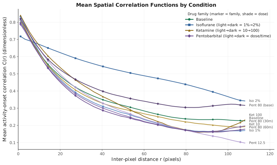
Figure N1: Spatial correlation C(r) as a function of inter-pixel distance for each condition. Nearby pixels are more correlated than distant ones; ξ is the characteristic distance over which that correlation decays. The curves shift vertically (different correlation floors and amplitudes) while maintaining similar decay lengths.
The Null Result
Across fifty recordings (four of the fifty-four were flagged as outliers in Curic’s metadata and excluded), spanning metabolic rates from 30% to 110% of awake baseline, the spatial correlation length did not vary. The metabolic rate Φ assigned to each condition is a calibrated estimate drawn from the anesthesia literature. For isoflurane, the values come from cerebral-metabolism measurements in mice (Wei et al., 2024) and humans (Alkire et al., 1997). For pentobarbital, they come from the barbiturate review of Slupe and Kirsch (2018). The two ketamine conditions sit apart. The lower dose (10 mg/kg) reaches the 110% upper end, because ketamine can raise cortical metabolism rather than suppress it (Langsjö et al., 2005); the higher dose (100 mg/kg) is assigned 75%. That non-monotonic metabolic response makes them unsuitable for a clean power-law fit, so they are omitted from the table below while remaining in the full nine-condition comparison that follows. The ninth condition, the pre-injection baseline of the paired pentobarbital series (Φ = 1.00, ξ = 22.0 ± 1.8), is also left out of the table; it returns in the paired analysis below.
| Condition | Metabolic rate (Φ) | ξ (pixels, mean ± SEM) |
|---|---|---|
| Awake baseline | 1.00 | 23.7 ± 1.8 |
| Isoflurane 1% | 0.60 | 19.6 ± 0.8 |
| Isoflurane 2% | 0.40 | 34.7 ± 3.7 |
| Pentobarbital 12.5 mg/kg | 0.80 | 23.5 ± 4.6 |
| Pentobarbital 80 mg/kg, 30 min | 0.35 | 21.5 ± 0.9 |
| Pentobarbital 80 mg/kg, 60 min | 0.30 | 20.1 ± 0.6 |
Power-law fit: ν = −0.0002, R2 < 0.001, p = 0.999. Bootstrap 95% confidence interval: [−0.09, +0.10]. ξ does not track metabolic rate.
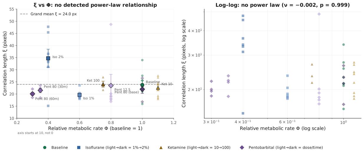
Figure N2: The flatline: ξ does not track metabolic rate. Each point is one recording; colors and shapes indicate drug class. The dashed line marks the grand mean, ξ = 24.0 pixels; the fitted power law is flat (ν = −0.0002, p = 0.999). Isoflurane 2% (burst suppression) is the one condition that stands apart.
Susceptibility told the same story. χ1D: ν = −0.04, p = 0.81. χ2D: ν = −0.09, p = 0.71. Neither susceptibility variant scales with metabolic rate.
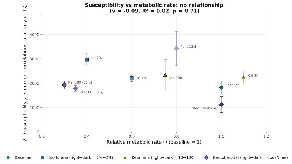
Figure N3: Susceptibility χ2D versus metabolic rate. Like ξ, the integrated excess correlation shows no systematic scaling with energy throughput.
One condition stands out: isoflurane at 2% produces ξ = 34.7, about 46% longer than the baseline. It is the most informative point in the entire analysis, and we return to it below.
What Does Vary
A Kruskal-Wallis test (comparing groups without assuming a particular distribution shape) across all nine conditions reveals which observables respond to anesthesia and which do not:
| Observable | Test statistic | p-value |
|---|---|---|
| ξ (correlation length) | 13.2 | 0.11 (not significant) |
| Susceptibility | 17.3 | 0.027 |
| Correlation floor (C∞) | 26.1 | 0.001 |
| Correlation amplitude | 27.4 | 0.0006 |
| Spike rate | 41.2 | 0.000002 |
Correlation length is the one observable that does not differ between conditions. Everything else changes with anesthetic state: susceptibility, correlation floor, correlation amplitude, spike rate. Susceptibility differs between conditions without tracking Φ. Spatial reach stays constant.
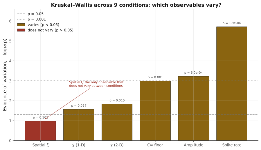
Figure N4: Which observables respond to anesthesia? Bar heights show the evidence of variation between conditions as −log10(p) from Kruskal-Wallis tests (taller = stronger evidence). The dashed line marks p = 0.05 and the dotted line p = 0.001. ξ is the only observable that does not differ.
Think of a road network. The roads have a characteristic length: how far you can drive before hitting the edge of town. Anesthesia changes the traffic, how many cars, how fast they move, whether they clump or spread, while leaving the roads untouched. Correlation length measures the roads. The DCP predicts the traffic.
Confirmation, One Mouse at a Time
Curic’s design included a paired component. Four mice were each recorded at baseline (pre-injection), thirty minutes after pentobarbital 80 mg/kg, and sixty minutes after. Each animal was measured under three metabolic states, eliminating between-subject variability. (The Friedman test below is the paired counterpart of the earlier Kruskal-Wallis comparison: the same question, asked within each animal rather than across groups.)
The paired analysis confirms the pooled result at the individual-animal level. In all four mice, pentobarbital drops the correlation floor (C∞ decreases, Friedman p = 0.039) and raises correlation amplitude (Friedman p = 0.018). The drug peels away a background haze of global synchrony, leaving local correlation sharper, as fog clearing reveals the contours of a landscape. Spike rate rises in all four animals, the increase near the threshold of significance (Friedman p = 0.050).
The correlation length ξ: two mice up, two mice down. Friedman p = 0.78. Even within individual animals undergoing a threefold metabolic suppression, the spatial reach does not budge.
The Burst-Suppressed Cortex
Isoflurane at 2% is the exception that tests the rule. At this dose, the drug forces the cortex into burst suppression: synchronous oscillations where vast swaths of tissue fire in lockstep, followed by silent periods where nothing fires. The cortex has been pharmacologically seized. Think of a command economy where every factory produces the same product on the same schedule. The central authority has removed every alternative.
The numbers tell the story. Isoflurane 2% has the longest correlation length in the dataset (ξ = 34.7) and the highest correlation floor (C∞ = 0.37, meaning distant pixel pairs retain a Pearson correlation of 0.37 regardless of separation).
Within the isoflurane dose series, the 2D susceptibility χ2D increases as metabolic rate decreases: 1,821 → 2,205 → 2,970, a rise of 63% from the awake cortex to the burst-suppressed one. The power-law fit gives ν = −0.53 with R2 = 0.96, though it rests on only three condition means (p = 0.12) and describes a trend rather than an established law. The negative sign means more suppression produces more apparent coordination. A negative ν is the signature of imposed coordination, the same sign the fixed-Hamiltonian spin chain gives (−0.40), and here a drug supplies it on demand: the order in a burst-suppressed cortex is administered rather than grown.
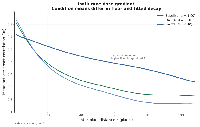
Figure N5: The isoflurane dose series, from baseline (green) through 1% (light blue) to 2% (dark blue, burst suppression). All three curves decay with distance, and the 1% curve settles slightly below baseline at long range. At 2%, the burst-suppressed cortex holds the strongest long-range correlation, with the highest floor and the longest fitted decay length.
The resulting “coordination” is long-range, high-amplitude, and brittle. Burst suppression alternates between synchronous firing and silence: a state incompatible with sustained computation.
Compare the awake cortex, which sustains lower-amplitude, shorter-range coordination indefinitely. It adjusts its patterns moment by moment in response to sensory input, memory retrieval, and internal computation. Less striking in a snapshot; incomparably more capable over time.
Two Correlation Lengths in One Dataset
The puzzle resolves when we recognize that Curic’s dataset contains two different kinds of “correlation length,” measured through two different windows.
The spatial correlation length comes from the decay of C(r), the curve showing how correlation falls off with physical distance. Two patches of cortex can only march together if some fiber carries the signal between them, so the distance at which correlation dies away reports the physical span of the wiring. It measures the reach of anatomical connections: lateral fibers within the cortex, callosal tracts (the thick cable connecting the two hemispheres), and thalamocortical loops (circuits relaying signals through deep-brain nuclei back to the surface). These connections do not change when an anesthetic is administered. They are the roads.
The dynamical correlation length comes from avalanche statistics: measurements of how activity cascades ripple across the network, the way a toppling domino propagates a fall down a line of dominoes. The critical exponents tau and alpha (mathematical signatures describing the size and duration distributions of these cascades) shift systematically with anesthetic depth. They describe how the traffic organizes.
One mechanism contributing to this traffic is ephaptic coupling (Chapter 17): each neuron’s firing generates an electromagnetic field that perturbs its neighbors without any synaptic connection. This shapes cascade propagation in real time. Activation patterns are either scale-free (near criticality, cascades of all sizes, long dynamical ξ) or truncated (away from criticality, only small cascades, short dynamical ξ). Cascade size is itself a measure of reach: a cascade that dies after three pixels has coordinated three pixels, while one that crosses the cortex has coordinated the cortex.
Reading the exponents therefore reads the dynamical ξ at one remove. The author’s ongoing analysis, using these critical exponents as a proxy for the dynamical correlation length, yields ν = +0.64 ± 0.07: positive and in the direction the principle predicts. This proxy estimate is preliminary; it infers the dynamical reach from the exponents rather than measuring it directly, and the value sits above the mean-field expectation of about +0.50.
Same brain. Same anesthetic conditions. Same dataset. The spatial observable gives ν ≈ 0. The dynamical observable gives ν > 0. The DCP applies to the traffic, not the roads.
| Observable | What it measures | Set by | ν |
|---|---|---|---|
| Spatial ξ (this analysis) | Anatomical reach of connections | Fixed wiring | ≈ 0 |
| Dynamical ξ (exponent proxy) | Distance from criticality | Activity-dependent dynamics | +0.64 |
The Classification Sharpens
This result fits into the progression across scales. The quantum spin-chain exponents come from the simulations in Chapter 17; the social values come from the World Values Survey trust regression (109 countries) and the firm-size analysis discussed there; the neural rows are the present analysis.
| System | Coupling type | ν |
|---|---|---|
| Quantum spin chain (fixed Hamiltonian) | Imposed | −0.40 |
| Quantum spin chain (Hebbian feedback) | Mixed | −0.14 |
| Neural cortex (spatial C(r)) | Fixed anatomical backbone | ≈ 0 |
| Neural cortex (dynamical exponents) | Activity-dependent | +0.64 |
| Social networks (World Values Survey trust) | Emergent, adaptive | +0.41 |
| Social institutions (firm size) | Emergent, adaptive | +0.38 |
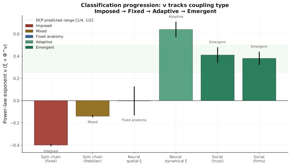
Figure N6: The sign and magnitude of ν track coupling type. Systems with fixed backbones (left) show ν ≤ 0; systems with adaptive, emergent coordination (right) show ν > 0. The neural data contributes both a null (spatial) and a positive (dynamical) result from a single physical system.
The sign and magnitude of ν track a single question: can the coordination network reorganize in response to energy throughput? Where the backbone is rigid (quantum lattice, cortical anatomy), ν is zero or negative; the structure was never free to adapt. Where network topology is itself a thermodynamic variable, growing and dissolving in response to dynamics, ν is positive: the signature the principle predicts for emergent coordination. The mean-field prediction (Chapter 17), which treats every element as feeling the averaged pull of all the others instead of only its immediate neighbors, places the expected exponent near +0.50 for systems where long-range links smooth out local structure. The social values (+0.41, +0.38) fall a little below that mark, and the neural dynamical proxy (+0.64 ± 0.07) a little above it.
Behind the positive sign is a simple economy: every link in an adaptive network costs energy to keep, so more throughput can sustain more links, and longer ones. Friendships form when people find value in each other and fade when they do not; adaptive networks reorganize the same way, their links sustained only as long as the dynamics reward them.
Previous evidence came from comparisons across disparate systems: quantum simulations versus cross-country surveys. The Curic data provides both results from a single physical system, one cortex, two observables, two regimes. The domain boundary runs through the middle of the brain.
What This Means for the Prediction
The ξ ~ Φν prediction refers to the dynamical correlation length: the range over which activity patterns organize adaptively. The mechanisms involved can strengthen, weaken, form, or dissolve in response to energy flux, as trade routes open when commerce is profitable and close when it is not.
In systems where network topology is adaptive (social networks, local neural circuits with Hebbian plasticity, ecosystems with mutualistic coupling), the spatial and dynamical correlation lengths should converge: the roads reshape themselves to match the traffic. Where a fixed anatomical backbone dominates (whole-cortex imaging, crystal lattices), the two lengths decouple.
The domain boundary sharpens the DCP. The principle applies to systems whose coordination is maintained by invitation: every link exists because the dynamics sustain it. Removing energy flux causes coordination to dissolve rather than merely fall silent.
Imposed Order Looks Stronger in a Snapshot
Imposed coordination looks more powerful than emergent coordination in a snapshot. The burst-suppressed cortex under isoflurane 2% produces the longest correlation length in the dataset. Measured by the range of synchronized activity at a single moment, coercion wins.
That impression dissolves when you ask what the coordinated system can do. The burst-suppressed cortex cannot process information, respond selectively to what it senses, form memories, generate predictions, or sustain computation. Every functional capacity has been sacrificed for the appearance of coordination.
The correlation length is one measurable axis of a difference that involves every aspect of neural processing.
The social parallel is structural. An authoritarian state can mobilize its entire population for a single purpose, producing impressive snapshots of coordinated action. A democracy, with its shorter “correlation length” of consensus, sustains adaptive governance over decades.
The Trust Attractor predicts that the democratic equilibrium is more thermodynamically stable. Invitation adjusts to perturbation; coercion can only double down or shatter. Burst suppression shows the same pattern physiologically: total synchrony alternating with total silence, no intermediate state available.
A snapshot measures reach. A trajectory measures resilience. The DCP is a statement about trajectories.
Data: Curic, D. et al. “Existence of multiple transitions of the critical state due to anesthetics.” Nat. Commun. 15, 7025 (2024). We thank Davor Curic for generously sharing the deconvolved calcium imaging data and for his expert guidance on spike detection from calcium indicators. Analysis scripts and results are available in the project repository.
Both are computed in
research/davor/susceptibility_and_within_drug.py. χ1D is the trapezoidal integral of the excess correlation over the fitted floor, ∫(C(r) − C∞) dr; χ2D carries the two-dimensional shell weighting, ∫2πr(C(r) − C∞) dr, the 2πr factor being the number of pixel pairs at each separation. Per-recording and per-condition values are inextended_analysis_results.npzalongside ξ, C∞, amplitude, and spike rate.↩︎